This was originally written for a talk at TFUG Kolkata. Read the slides here.

Introduction

Let's first talk a bit about message queues.

We see the word "queue" in it, why?

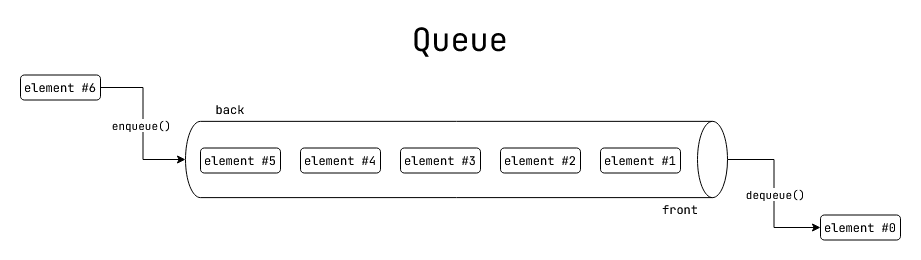
Fig: a First In First Out (FIFO) queue.

A queue is a first in first out data-structure for storing a set of elements.

However this definition doesn't tell us anything about:

• How and where the elements are stored (in-memory, hard disk etc.)
• Who can access this queue from where

In the 21st century, we have the following additional requirements:

• It has to be accessible over the internet over well known protocols (HTTP, gRPC etc.)
• It might need to implement role base access control (RBAC)
• It has to be persistent if necessary
• It has to be replicated to be highly available.
• All replicas need to be consistent with each other
• It has to support multiple channels for different types of elements
• It has to be reasonably fast
• We can't be bothered about these requirements. We have business requirements to worry about

Message queues are queues of "message" elements, and they fulfil the above requirements.

Message queue usage model

This section discusses the models of computations possible using message queues.

Background: Client Server model

Let us first discuss how we work without message queues.

In the conventional client server model, the client makes synchronous requests to the server, which responds back with a synchronous response.

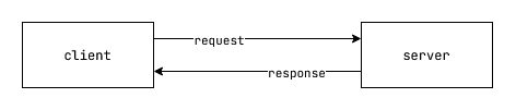
Fig: Client - Server model.

What happens when we have too many clients that the server can't handle at once?

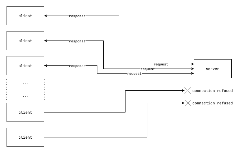
Fig: Client - Server model overhelmed with too many clients for the server to handle.

The server is simply unable to service all the clients within a reasonable time. Either the requests time out completely, or the server starts refusing connections when the maximum number of connections is reached. The server may also be also be configured with request rate limits where the server start dropping requests altogether if they arrive at a higher than expected rate.

Message Queue: Asynchronous processing

Message queues enable asynchronous handling of requests.

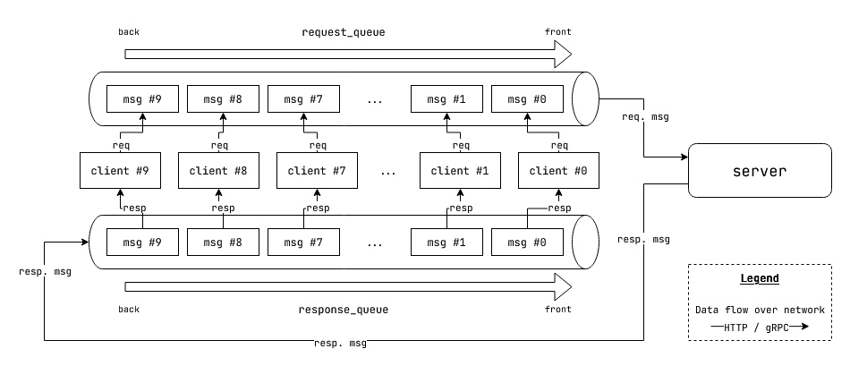
Fig: Asynchronous processing of requests with request and response queues.

Asynchronous processing allows the server to actually handle all the requests without timing out or refusing connections. However in this case, the responses are available later at a different time, as opposed to client - server model where responses are available synchronously.

However, this is not the only thing that message queues are good at. Message queues also enable large scale request handling with multiple stages, and horizontal scaling at each stage. But how?

Message Queue: Multi-stage horizontally scalable asynchronous processing

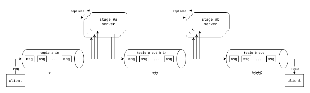
Fig: Multi-stage asynchornous horizontally scalable processing.

In the above figure, we have to stages of computation stage #a and stage #b. There are two sets of servers for hosting these stages of computation. These two stages are connected to each other with message queue topics. This architecture works as follows:

• Client pushes a message containing the input request to be processed into the first topic topic_a_in
• The stage #a server pulls in messages from the topic_a_in topic, processes it and writes the intermediate result to topic_a_out_b_in topic.
• The stage #b server pulls in intermeidate processed results from the topic_a_out_b_in topic, processes them and writes the final output to topic_b_out topic.
• The client reads the results from the topic_b_out topic.

You may also think of the stage #a and stage #b as two functions $a(x)$ and $b(x)$, and we are essentially computing the composite function $(b \circ a)(x) = b(a(x))$ where $x$ is the client input request. The difference being:

• The values are passed into the "function"(s) over the network via message queues
• There is a queue of values $X = \lbrace x_0, x_1, ...\rbrace $ to process.
• The invocation at every stage can be done in parallel with the stage replicas. The message queue is responsible for adequately load balancing the elements from the queue among all the replicas.

Now in order to see, how this load balancing is done in practice, let's take a look at two popular message queuing solutions:

• Apache Kafka
• Google Cloud Pub/Sub

Apache Kafka

In Apache Kafka, messages are organized by "topic"(s). Each "topic" is further broken down partitions. Messages in a partition are ordered and isolated from messages in another partition.

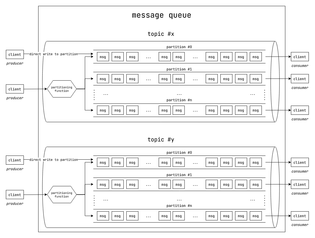
Fig: Topics and partitions in Apache Kafka.

There are two kinds of clients for Apache Kafka: Producers and Consumers

• Producers produce messages into a topic in Kafka. They can choose to write to a particular partition or let Kafka load balance messages to a partition.
• Consumers consume message from a particular partition under a topic.

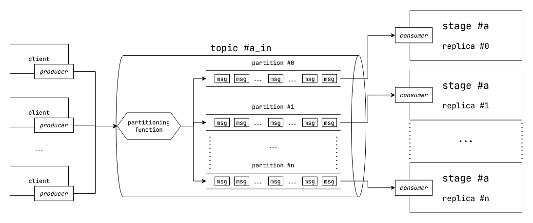
Fig: Horizontally scaling a stage with Kafka partitions.

In our multistage computation example, each stage has input request and output responses. Let's assign a particular topic to a particular stage. To achieve horizontal scaling we do the following:

• We make multiple partitions under the topic for this stage.
• We write input requests to the topic. The partitioner load balances the messages to the partitions under this topic.
• We run multiple instances of the request hander for this stage. Each stage contains a consumer which reads from a particular partition.
• In order to horizontally scale up further, we increase the number of partitions and request handler instances.

Google Cloud Pub/Sub

Google Cloud Pub/Sub makes this a bit more simpler. There are "topic"(s) where messages are written to. Each "topic" can have a set of "subscription"(s). There can be multiple publishers to a topic, and multiple subscribers that read from multiple subscriptions from the topic.

Message published to the topic are load balanced across all the subscriptions.

Primary distinction between synchronous and asynchronous request processing

• Synchronous model: Requests are delivered to the server as soon as they arrive. If the server has enough resources to handle the requests, they are processed. Otherwise they are either delayed or dropped.
• Asynchronous model: Requests are buffered as soon as they arrive. Then the server pulls a request from the buffered queue of requests when it has enough resources to handle the request. This improved the success rate of requests being handled successfully.

Some also call this event driven architecture, with the individual messages being "event"(s)

Why use message queues instead of Databases?

Why don't we use different tables for representing topics? Each row could be a message. We could use a partitioning function like modulus to partition the topic for horizontal scaling.

You can indeed do this, some production systems use databases instead of message queues in this manner.

However message queues have some advantages over traditional data bases:

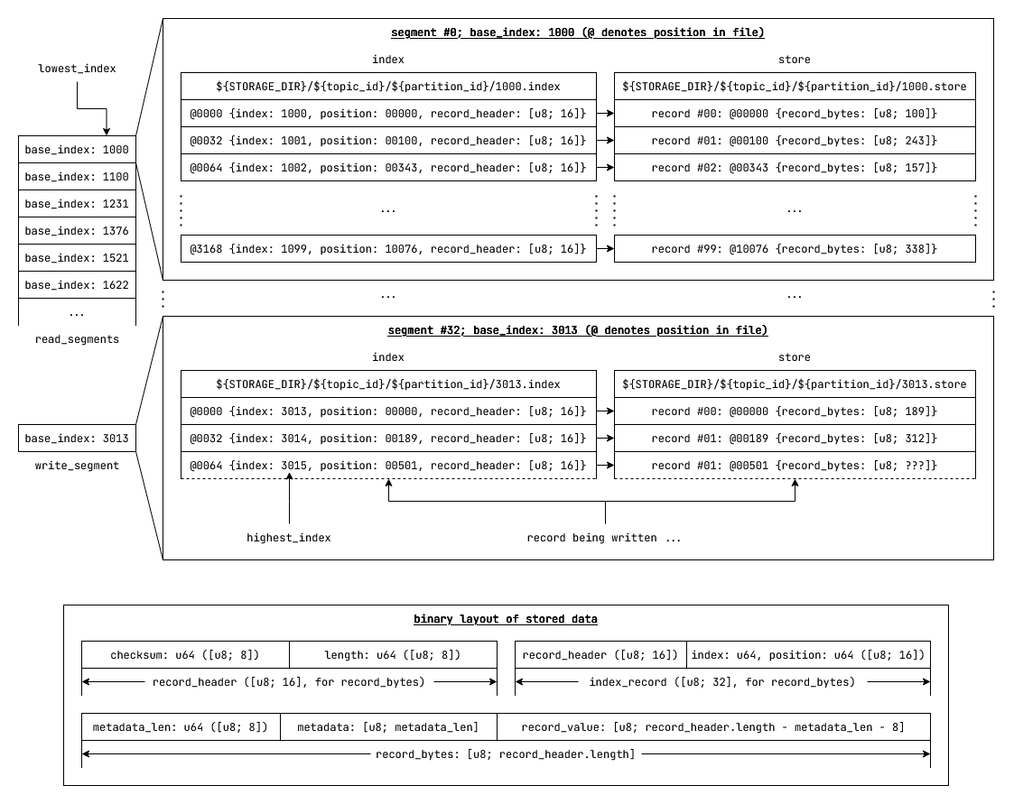
Fig: The segmented-log data-structure.

• Message queues use different data structures for storage and indexing. Message queues use segmented_log(s), while traditional relational databases use data-structures from the B-Tree family
• segmented_log and B-Tree performance comparison:
  • segmented_log(s) have $O(1)$ writes on average. B-Tree(s) have $O(\log n)$ insertions.
    • In segmented_log appending to the write_segment is $O(1)$
    • When rotating the write_segment, vector::push_back on vector of read segments is $O(1)$ on average, $O(|segments|)$ at worst.
    • Modern vector implementations ensure that the worst case of having to copy all the elements when pushing back to end of the vector is very rare. They may employ the following approaches:
      • Exponential memory reservation when reserving more memory
      • Maintaining multiple disjoint contiguous slabs of memory to avoid having to copy elements when reserving more memory. New elements are written to the last memory slab. This reduces worst case for push_back to almost $O(1)$ on average. Reads are still $O(1)$ since the memory region for any index can be easily computed as all elements have same size and the regions are identical in size.
  • segmented_log(s) can guarantee $O(\log |segments|)$ reads while B-Trees have $O(\log n)$ reads, where $n$ is the total number of records and $segments$ is the set of segments in the segmented_log. (Usually, $\frac{n}{|segments|} >= 1000$)
    • This is possible since the segments are sorted by indices and given a record index, we can perform a binary search to check which segment has the record with the index, which would be $O(\log |segments|)$. Reading at a specific index from a segment is $O(1)$.
    • If we can guarantee constant record size (with padding) and constant max number of records per segment, we can provide $O(1)$ reads for segmented_log(s). This would be possible because determining which segment has the index would also be a $O(1)$ in this case.

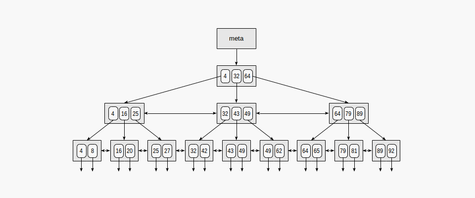
Fig: The B-Tree data-structure.

• segmented_log and B-Tree comparison continued ...
  • segmented_log(s) have far lesser number of memory indirections than B-Tree(s) when simply sequentially iterating over the elements. (Trees have multiple levels of pointer indirection, as opposed to vectors which have contiguous memory allocation and are very cache-friendly). Higher number of memory indirections increase the number of virtual memory page faults and decrease cache locality.
  • segmented_log(s) have higher disk page locality. This due to segmented_log's append only nature where writes always go to the end of the files, which is optimal for disk page cache.
  • segmented_log(s) are highly optimized on SSDs due to it's sequential append only write characteristics
  • In conclusion, segmented_log(s) support much faster writes and reads than B-Tree(s), on average.
• Modern databases that are based on LSM trees (Google BigTable, Google Spanner, Cassandra, DynamoDB, TiKV, Redis) have similar performance characteristics to segmented_log(s)
• Message queues don't require a query parsing and execution layer for accessing messages.
• Writes in databases often require transactions for atomicity and consistency guarantees. For distributed databases, there are distributed transactions with sophisticated protocols like two phase commit which blocks on failure. Message queues can rely on consensus algorithms like Raft and Paxos for consistency between replicas, which are non-blocking and more resilient to failures.
• Message queues have been explicitly designed to provide queue like semantics. One has to build additional abstractions over databases to obtain message queue like behaviour.

However, the gaps between message queues and databases are gradually decreasing. Apache Kafka now provides an SQL like query layer for stream analytics. In-memory key value stores (databases) like Redis also provide message queue abstractions out of the box.

Remember that this talk was actually about Machine Learning inference with message queues and not just about message queues. To illustrate how message queues might be used in a machine learning inference system in the real world, consider the following case study.

Case Study: Plant medicine effectiveness on Crops

An agricultural pharmacy company has come up with a new drug to cure various plant diseases. Now, they wish to measure the effectiveness of their medicine. They want to quantitatively analyze if the medicine speeds up the healing process in plants.

In order to to do this, the company partners with a farm owner to test out the medicine on their crops. They isolate the farm into two areas, the control area where no medicine is used and the active area where the newly developed medicine is tested out. They decide on a uniform medicine distribution quantity, let's say 120 ml/sqft.

Now they employ a fleet of drones to regularly take images of the plants in the farm in both the control and active areas to keep track of the health of the plants. The drones take photographs of the plants in the farm at regular distances to cover the entire farm. The trajectory of the drones are preprogrammed in such way that each drones always take photographs at some specific positions (marked by GPS) and each photograph contains a maximum of 20 leaves. The drones take photographs at regular time intervals (e.g daily)

(The plants are in a green house. They don't move around a lot due to absence of wind)

The Machine Learning engineers are to analyze the photographs taken by the drones and measure the effect of the medicine on the leaves.

Now take a look at this photograph:

Fig: A plant suffering from a fungal-attack.

Intuitively it makes sense that if the disease progresses, the disease affected area will spread and increase. If it heals, the disease area will decrease.

The excellent machine learning engineers in this room would agree that approaching this problem with semantic segmentation would be powerful. From a single image with multiple leaves, multiple disease types can be detected along with the area covered by each type.

However that is an ideal case. It is only possible if you have the required datasets.

The machine learning engineers only have the following datasets:

• Leaf object detection dataset
• Disease grade classification for 5 diseases (the grades correspond to severity)

There are no sufficiently large annotated semantic segmentation dataset that can be used for production purposes. (Let's say, for this scenario.)

Solution Architecture

The machine learning engineers provide the following models:

• A leaf object detector
• 5 disease grade classifier models. Each disease grade classifier models has 4 classes.

The software engineers design the solution with a suite of micro-services and drone controllers which communicate with each other using the message queue.

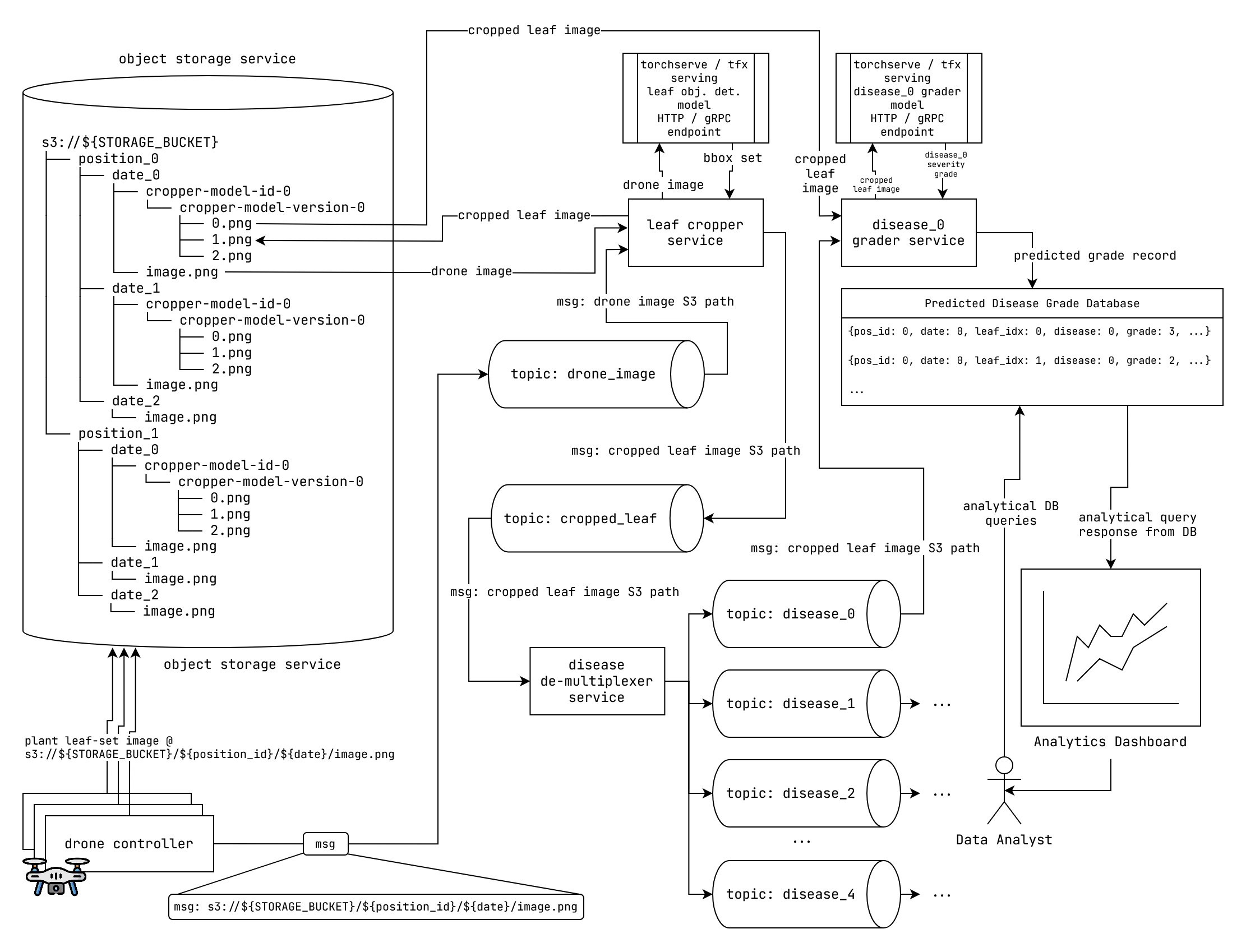
Fig: Solution Architecture diagram.

The main steps are as follows:

• Leaf obj detection on plant image
• Leaf bounding box detection
• Leaf image Crop from detected bounding boxes
• Disease grade classification on individual cropped leaf images
• Store prediction in DB
• Aggregate Queries for insights

The various components of the system are described in the following sections.

Drone Image Collector

The drone moves to specific position clicks an image, and uploads it to an S3/GCS bucket at a specific path. Each drone position has a unique identifier. The image path could be of the form:

s3://${STORAGE_BUCKET}/${position_id}/${date}/image.png

Next the drone controller produces a message on the "drone_image" topic. The message simply contains the S3 image object path.

We assume that the drones are equipped with some form of internet connectivity.

In the following section, when I say that a components consumes a message, if the message contains an image url, assume that the component also downloads the image from the url to it's local storage.

Also the service might use a shared persistent storage service to avoid hitting S3 every time.

Leaf image cropper

The leaf image cropper crops out the leaves from the drone image using the leaf object detection model.

The leaf object detection is model is served with a model serving solution like "Tensorflow serving" or "PyTorch serve". The model serving solution provides the model inference at specific HTTP or gRPC endpoint.

The leaf image cropper has a consumer to consume drone image from the "drone_image" topic. It then perform inference with the HTTP or gRPC endpoint served by the model serving solution and obtains all the bounding boxes. It then uses bounding boxes to crop out the leaves.

For each cropped out leaf:

• A new cropped leaf image is created. It is uploaded to:

  s3://${STORAGE_BUCKET}/${position_id}/${date}/${cropper-model-id}/${cropper-model-version}/${leaf_crop_idx}.png
  

• It produces a message on the "cropped_leaf" topic. The message contains the above S3 image object path.

Disease demultiplexer service

This service simply consumes a message from the "cropped_leaf" and produces it on each of the 5 disease grader topics "disease_0", "disease_1", ..., "disease_4".

This service might not be necessary in some message queues where they provide utilities to do this automatically.

Individual disease grader services

Each disease has 4 grades with 0 for healthy and 4 for most severe.

A disease grader service uses it's corresponding disease grading model to grade the severity of the cropped leaf for the corresponding disease.

The "disease_#n" grader model is served with a model serving solution like "Tensorflow serving" or "PyTorch serve". The model serving solution provides the model inference at specific HTTP or gRPC endpoint.

A disease grader service consumes a cropped leaf image from it's corresponding input topic, performs inference with the HTTP or gRPC endpoint exposed by the model serving solution, and writes a record with the following schema to a database:

{
  position_id: …, // drone position on field
  date: …, // date on which image was taken
  leaf_crop_idx: …, // leaf crop index from leaf crops with obj. det. model
  disease_type: …, // disease grader disease type
  predicted_grade: …, // predicted disease severity grade
  cropper_model_id: …, // model used for cropping
  cropper_model_version: … // version of cropper model used
  disease_model_id: …, // model used for predicting disease
  disease_model_version: …, // version of the disease predictor model used
}

Data Analysis

Once we have the leaf disease prediction data, a competent Data Analyst can use different analytical queries to obtain insights about the efficiency of the medicine. There can also be an analytical service which runs in the background and recomputes a set of analytical queries to maintain a set of dashboards.

Audits and Reproducibility

You might have observed that we also store the model id and version with each record. This is necessary if we need to re-analyze with different versions of different models.

We can regenerate all the messages by walking over the contents of the message queue and the system will perform inference as necessary. However, some message queues (like Apache Kafka) also allow you to replay messages.

For instance, consider we updated the model for "disease_3" and we want to re-analyze the images. We may simply replay the messages in the topic for "disease_3" along with new model config for the corresponding disease grader service. This will produce new disease inference records with the appropriate model details.

Scaling up horizontally

Now as discussed toward the start of the talk, individual services can be horizontally scaled easily. In our scenario the object detection service could using a model like MobileNet which has faster inference times, but the classifier service might be using a ResNet for classification which has slower inference times.

As we already know, a system is only as fast as the slowest component in the system. So in this example, we would need to create more replicas of the ResNet classifier service.

Now the model prediction endpoint and the web service communicate over the network. So they can be scaled independently if necessary. For instance, we might not choose to scale up the web component of a disease grader service, but we can increase the number of model replicas in the model serving solution instead (PyTorch serve for instance.) Also it is not necessary that the web components each have their unique instance of the model serving solution. They could all make requests to shared model serving solution instance.

Support for multiple environments

Now in this design itself, we don't specify whether the services are containers, pods in k8s or simple linux processes. As long as they communicate with each other on the message queue, it doesn't matter where they run.

This flexibility allows us to pursue multi-cloud architectures where different components could be running on different service clouds (some on GCP, some on AWS etc.). At the same time, this entire system could simply run on just a beefy laptop, albeit with some loss of throughput.

Conclusion

Message Queues act as a general communication layer between different cooperating web services. They enable asynchronous processing of requests, horizontal scaling at each layer and higher capacity for handling requests. These properties make them an excellent communication layer between different Machine Learning inference services.